AIML for Data Science

- Assignment 1 Submit here
- Types of Regression
- Types of classification
- Concept of underfitting and overfitting
- KNN
- Decision trees and unsupervised learning
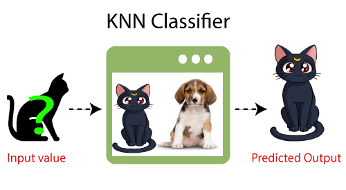
K-Nearest Neighbor(KNN) Algorithm for Machine Learning
- K-Nearest Neighbour is one of the simplest Machine Learning algorithms based on Supervised Learning technique.
- K-NN algorithm assumes the similarity between the new case/data and available cases and put the new case into the category that is most similar to the available categories.
- K-NN algorithm stores all the available data and classifies a new data point based on the similarity. This means when new data appears then it can be easily classified into a well suite category by using K- NN algorithm.
- K-NN algorithm can be used for Regression as well as for Classification but mostly it is used for the Classification problems.
- K-NN is a non-parametric algorithm, which means it does not make any assumption on underlying data.
- It is also called a lazy learner algorithm because it does not learn from the training set immediately instead it stores the dataset and at the time of classification, it performs an action on the dataset.
- KNN algorithm at the training phase just stores the dataset and when it gets new data, then it classifies that data into a category that is much similar to the new data.
- Example: Suppose, we have an image of a creature that looks similar to cat and dog, but we want to know either it is a cat or dog. So for this identification, we can use the KNN algorithm, as it works on a similarity measure. Our KNN model will find the similar features of the new data set to the cats and dogs images and based on the most similar features it will put it in either cat or dog category.
Why do we need a K-NN Algorithm?
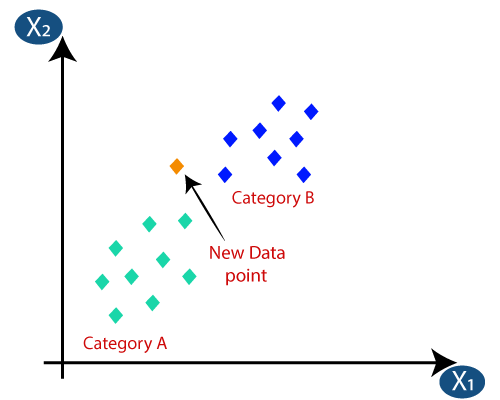
Suppose there are two categories, i.e., Category A and Category B, and we have a new data point x1, so this data point will lie in which of these categories. To solve this type of problem, we need a K-NN algorithm. With the help of K-NN, we can easily identify the category or class of a particular dataset. Consider the below diagram:
How does K-NN work?
The K-NN working can be explained on the basis of the below algorithm:
- Step-1: Select the number K of the neighbors
- Step-2: Calculate the Euclidean distance of K number of neighbors
- Step-3: Take the K nearest neighbors as per the calculated Euclidean distance.
- Step-4: Among these k neighbors, count the number of the data points in each category.
- Step-5: Assign the new data points to that category for which the number of the neighbor is maximum.
- Step-6: Our model is ready.
Suppose we have a new data point and we need to put it in the required category. Consider the below image:
- Firstly, we will choose the number of neighbors, so we will choose the k=5.
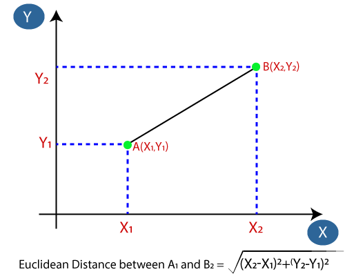
- Next, we will calculate the Euclidean distance between the data points. The Euclidean distance is the distance between two points, which we have already studied in geometry. It can be calculated as:
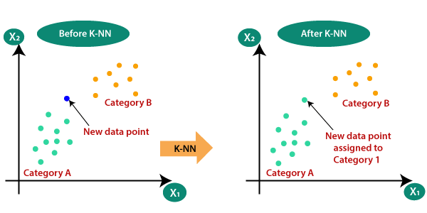
- By calculating the Euclidean distance we got the nearest neighbors, as three nearest neighbors in category A and two nearest neighbors in category B. Consider the below image:
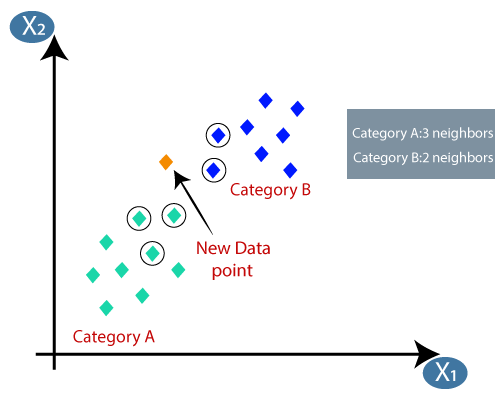
- As we can see the 3 nearest neighbors are from category A, hence this new data point must belong to category A.
Preprocessing refers to the steps taken to prepare data for use in machine learning models. These steps can include a variety of techniques such as data cleaning, feature extraction, and feature scaling. Preprocessing and scaling are essential steps in data preprocessing before applying any machine learning algorithm. The main goal of preprocessing is to transform the raw data into a format that is easier to analyze and model.
Scaling is a common preprocessing technique that involves transforming the numerical features of a dataset so that they are on a similar scale. This can help improve the performance of certain machine learning models, particularly those that are sensitive to differences in the magnitude of features.
There are several different kinds of preprocessing techniques, including:
Data cleaning: This involves removing or correcting any errors, missing values, or outliers in the data.
Feature extraction: This involves transforming raw data into a set of features that are more useful for machine learning models. This can include techniques such as PCA (Principal Component Analysis), LDA (Linear Discriminant Analysis), and feature selection.
Feature scaling: This involves transforming the numerical features of a dataset so that they are on a similar scale. This can include techniques such as standardization (subtracting the mean and dividing by the standard deviation) or normalization (scaling the values to a range between 0 and 1).
Data augmentation: This involves generating new training data by applying transformations to the existing data. This can be useful for improving the robustness of machine learning models.
Data integration: Combining multiple datasets into a single one.
Data transformation: Converting data from one format to another, such as normalizing or standardizing data.
Data reduction: Reducing the size of the dataset by selecting a subset of features or instances.
Data discretization: Converting continuous data into discrete intervals
Applying Data Transformations:
When applying data transformations, it is important to scale the training and test data in the same way. This ensures that the model is not biased towards one dataset or the other.
The effect of preprocessing on supervised learning can be significant. For example, feature scaling can improve the performance of models that use distance-based algorithms (such as k-NN and SVMs), while feature selection can help to reduce overfitting in models that have a large number of features. Overall, preprocessing can help to improve the accuracy and generalization of machine learning models. Data transformations involve scaling or normalizing the data to bring all features onto the same scale. Common techniques include:
Min-Max Scaling: Rescaling features to a range between 0 and 1.
Standardization: Scaling features to have a mean of 0 and a standard deviation of 1.
Log Transformation: Applying a log function to features to reduce the impact of outliers.
Scaling Training and Test Data the Same Way:
It is important to scale the training and test data in the same way to avoid data leakage. This means using the same scaling parameters (such as mean and standard deviation) for both sets.
The Effect of Preprocessing on Supervised Learning:
Preprocessing can have a significant impact on the performance of a supervised learning algorithm. By cleaning, transforming, and scaling the data, we can improve the accuracy and reduce overfitting. However, if the preprocessing steps are not appropriate for the data, they can also lead to poor performance. Therefore, it is important to carefully choose and evaluate the preprocessing steps for each dataset and problem.
PCA (Principal Component Analysis) and LDA (Linear Discriminant Analysis) are both commonly used techniques for feature extraction and dimensionality reduction in machine learning and data analysis. However, they have different goals and approaches.
PCA is a technique that is used to identify patterns in data by reducing the number of dimensions. It works by finding the directions of maximum variance in the data and projecting the data onto these directions. The resulting components are ordered in terms of the amount of variance they explain. PCA is an unsupervised learning technique, meaning it doesn't use any information about the class labels of the data.
LDA, on the other hand, is a supervised learning technique used to find the directions that maximize the separation between different classes in the data. It works by projecting the data onto a lower-dimensional space while maximizing the class separation. In LDA, the class labels of the data are used to find the directions that best discriminate between the different classes.
In summary, the main differences between PCA and LDA are:
Goal: PCA is used to reduce the number of dimensions in data while retaining the maximum amount of information, while LDA is used to find the directions that maximize the separation between different classes.
Supervision: PCA is an unsupervised technique, while LDA is a supervised technique.
Dimensionality reduction: PCA reduces the number of dimensions by finding the directions of maximum variance, while LDA finds the directions that best discriminate between the different classes.
K-Means Clustering Algorithm
K-Means Clustering is an unsupervised learning algorithm that is used to solve the clustering problems in machine learning or data science. In this topic, we will learn what is K-means clustering algorithm, how the algorithm works, along with the Python implementation of k-means clustering.
What is K-Means Algorithm?
K-Means Clustering is an Unsupervised Learning algorithm, which groups the unlabeled dataset into different clusters. Here K defines the number of pre-defined clusters that need to be created in the process, as if K=2, there will be two clusters, and for K=3, there will be three clusters, and so on.
It is an iterative algorithm that divides the unlabeled dataset into k different clusters in such a way that each dataset belongs only one group that has similar properties.
It allows us to cluster the data into different groups and a convenient way to discover the categories of groups in the unlabeled dataset on its own without the need for any training.
It is a centroid-based algorithm, where each cluster is associated with a centroid. The main aim of this algorithm is to minimize the sum of distances between the data point and their corresponding clusters.
The algorithm takes the unlabeled dataset as input, divides the dataset into k-number of clusters, and repeats the process until it does not find the best clusters. The value of k should be predetermined in this algorithm.
The k-means clustering algorithm mainly performs two tasks:
- Determines the best value for K center points or centroids by an iterative process.
- Assigns each data point to its closest k-center. Those data points which are near to the particular k-center, create a cluster.
Hence each cluster has datapoints with some commonalities, and it is away from other clusters.
The below diagram explains the working of the K-means Clustering Algorithm:
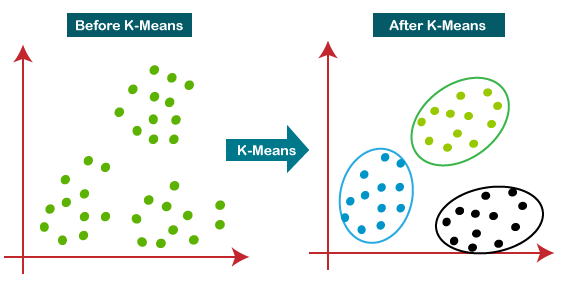
How does the K-Means Algorithm Work?
The working of the K-Means algorithm is explained in the below steps:
Step-1: Select the number K to decide the number of clusters.
Step-2: Select random K points or centroids. (It can be other from the input dataset).
Step-3: Assign each data point to their closest centroid, which will form the predefined K clusters.
Step-4: Calculate the variance and place a new centroid of each cluster.
Step-5: Repeat the third steps, which means reassign each datapoint to the new closest centroid of each cluster.
Step-6: If any reassignment occurs, then go to step-4 else go to FINISH.
Step-7: The model is ready.
Let's understand the above steps by considering the visual plots:
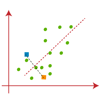
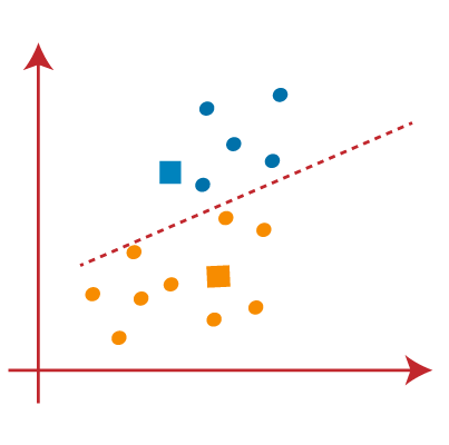
Suppose we have two variables M1 and M2. The x-y axis scatter plot of these two variables is given below:
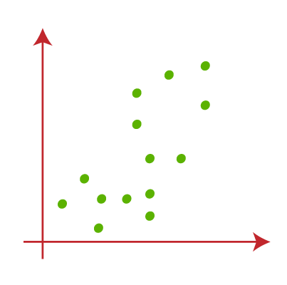
- Let's take number k of clusters, i.e., K=2, to identify the dataset and to put them into different clusters. It means here we will try to group these datasets into two different clusters.
- We need to choose some random k points or centroid to form the cluster. These points can be either the points from the dataset or any other point. So, here we are selecting the below two points as k points, which are not the part of our dataset. Consider the below image:
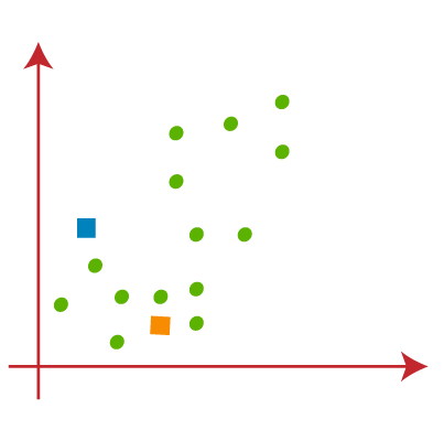
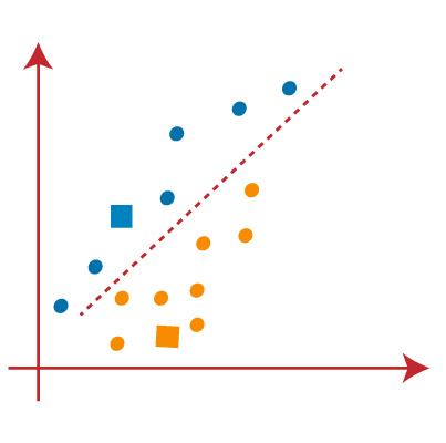
- Now we will assign each data point of the scatter plot to its closest K-point or centroid. We will compute it by applying some mathematics that we have studied to calculate the distance between two points. So, we will draw a median between both the centroids. Consider the below image:
From the above image, it is clear that points left side of the line is near to the K1 or blue centroid, and points to the right of the line are close to the yellow centroid. Let's color them as blue and yellow for clear visualization.
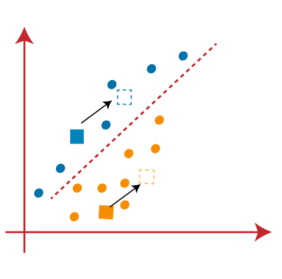
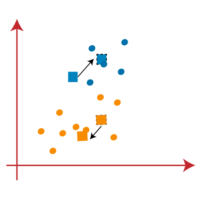
- As we need to find the closest cluster, so we will repeat the process by choosing a new centroid. To choose the new centroids, we will compute the center of gravity of these centroids, and will find new centroids as below:
- Next, we will reassign each datapoint to the new centroid. For this, we will repeat the same process of finding a median line. The median will be like below image:
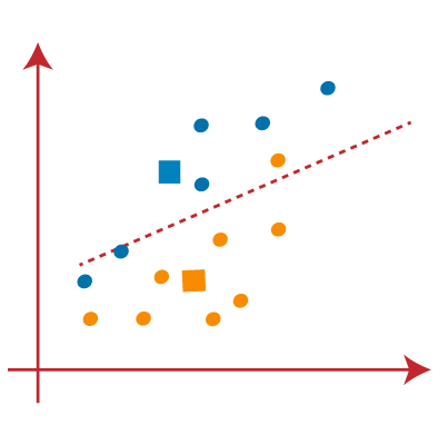
From the above image, we can see, one yellow point is on the left side of the line, and two blue points are right to the line. So, these three points will be assigned to new centroids.
As reassignment has taken place, so we will again go to the step-4, which is finding new centroids or K-points.
- We will repeat the process by finding the center of gravity of centroids, so the new centroids will be as shown in the below image:
- As we got the new centroids so again will draw the median line and reassign the data points. So, the image will be:
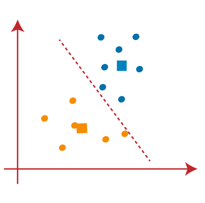
- We can see in the above image; there are no dissimilar data points on either side of the line, which means our model is formed. Consider the below image:
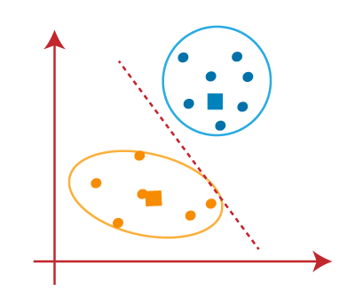
As our model is ready, so we can now remove the assumed centroids, and the two final clusters will be as shown in the below image:
How to choose the value of "K number of clusters" in K-means Clustering?
The performance of the K-means clustering algorithm depends upon highly efficient clusters that it forms. But choosing the optimal number of clusters is a big task. There are some different ways to find the optimal number of clusters, but here we are discussing the most appropriate method to find the number of clusters or value of K. The method is given below:
Elbow Method
The Elbow method is one of the most popular ways to find the optimal number of clusters. This method uses the concept of WCSS value. WCSS stands for Within Cluster Sum of Squares, which defines the total variations within a cluster. The formula to calculate the value of WCSS (for 3 clusters) is given below:
In the above formula of WCSS,
∑Pi in Cluster1 distance(Pi C1)2: It is the sum of the square of the distances between each data point and its centroid within a cluster1 and the same for the other two terms.
To measure the distance between data points and centroid, we can use any method such as Euclidean distance or Manhattan distance.
To find the optimal value of clusters, the elbow method follows the below steps:
- It executes the K-means clustering on a given dataset for different K values (ranges from 1-10).
- For each value of K, calculates the WCSS value.
- Plots a curve between calculated WCSS values and the number of clusters K.
- The sharp point of bend or a point of the plot looks like an arm, then that point is considered as the best value of K.
Since the graph shows the sharp bend, which looks like an elbow, hence it is known as the elbow method. The graph for the elbow method looks like the below image:
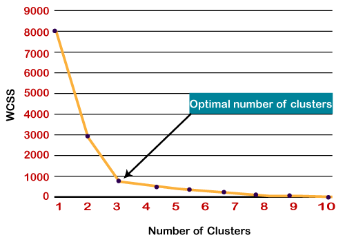
Note: We can choose the number of clusters equal to the given data points. If we choose the number of clusters equal to the data points, then the value of WCSS becomes zero, and that will be the endpoint of the plot.
Python Implementation of K-means Clustering Algorithm
In the above section, we have discussed the K-means algorithm, now let's see how it can be implemented using Python.
Before implementation, let's understand what type of problem we will solve here. So, we have a dataset of Mall_Customers, which is the data of customers who visit the mall and spend there.
In the given dataset, we have Customer_Id, Gender, Age, Annual Income ($), and Spending Score (which is the calculated value of how much a customer has spent in the mall, the more the value, the more he has spent). From this dataset, we need to calculate some patterns, as it is an unsupervised method, so we don't know what to calculate exactly.
The steps to be followed for the implementation are given below:
- Data Pre-processing
- Finding the optimal number of clusters using the elbow method
- Training the K-means algorithm on the training dataset
- Visualizing the clusters
Step-1: Data pre-processing Step
The first step will be the data pre-processing, as we did in our earlier topics of Regression and Classification. But for the clustering problem, it will be different from other models. Let's discuss it:
- Importing Libraries
As we did in previous topics, firstly, we will import the libraries for our model, which is part of data pre-processing. The code is given below:
In the above code, the numpy we have imported for the performing mathematics calculation, matplotlib is for plotting the graph, and pandas are for managing the dataset.
- Importing the Dataset:
Next, we will import the dataset that we need to use. So here, we are using the Mall_Customer_data.csv dataset. It can be imported using the below code:
By executing the above lines of code, we will get our dataset in the Spyder IDE. The dataset looks like the below image:
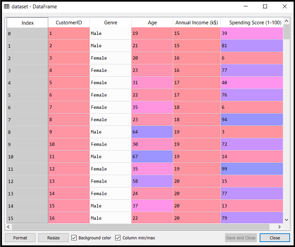
From the above dataset, we need to find some patterns in it.
- Extracting Independent Variables
Here we don't need any dependent variable for data pre-processing step as it is a clustering problem, and we have no idea about what to determine. So we will just add a line of code for the matrix of features.
As we can see, we are extracting only 3rd and 4th feature. It is because we need a 2d plot to visualize the model, and some features are not required, such as customer_id.
Step-2: Finding the optimal number of clusters using the elbow method
In the second step, we will try to find the optimal number of clusters for our clustering problem. So, as discussed above, here we are going to use the elbow method for this purpose.
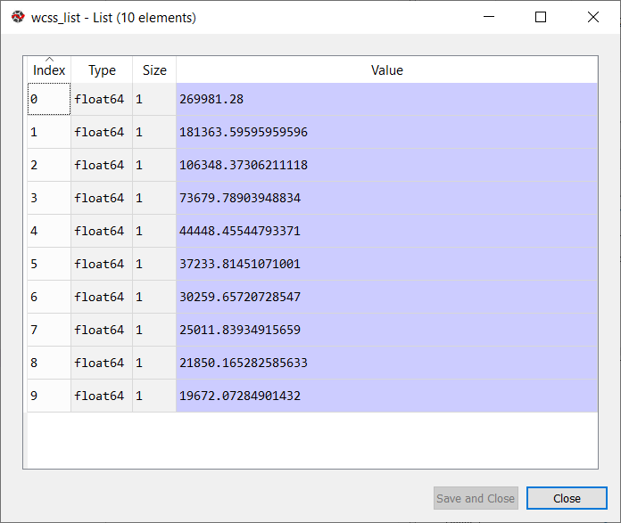
As we know, the elbow method uses the WCSS concept to draw the plot by plotting WCSS values on the Y-axis and the number of clusters on the X-axis. So we are going to calculate the value for WCSS for different k values ranging from 1 to 10. Below is the code for it:
As we can see in the above code, we have used the KMeans class of sklearn. cluster library to form the clusters.
Next, we have created the wcss_list variable to initialize an empty list, which is used to contain the value of wcss computed for different values of k ranging from 1 to 10.
After that, we have initialized the for loop for the iteration on a different value of k ranging from 1 to 10; since for loop in Python, exclude the outbound limit, so it is taken as 11 to include 10th value.
The rest part of the code is similar as we did in earlier topics, as we have fitted the model on a matrix of features and then plotted the graph between the number of clusters and WCSS.
Output: After executing the above code, we will get the below output:
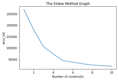
From the above plot, we can see the elbow point is at 5. So the number of clusters here will be 5.
Step- 3: Training the K-means algorithm on the training dataset
As we have got the number of clusters, so we can now train the model on the dataset.
To train the model, we will use the same two lines of code as we have used in the above section, but here instead of using i, we will use 5, as we know there are 5 clusters that need to be formed. The code is given below:
The first line is the same as above for creating the object of KMeans class.
In the second line of code, we have created the dependent variable y_predict to train the model.
By executing the above lines of code, we will get the y_predict variable. We can check it under the variable explorer option in the Spyder IDE. We can now compare the values of y_predict with our original dataset. Consider the below image:
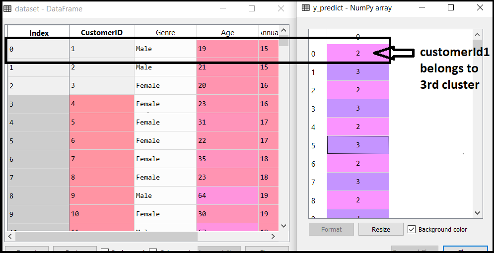
From the above image, we can now relate that the CustomerID 1 belongs to a cluster
3(as index starts from 0, hence 2 will be considered as 3), and 2 belongs to cluster 4, and so on.
Step-4: Visualizing the Clusters
The last step is to visualize the clusters. As we have 5 clusters for our model, so we will visualize each cluster one by one.
To visualize the clusters will use scatter plot using mtp.scatter() function of matplotlib.
In above lines of code, we have written code for each clusters, ranging from 1 to 5. The first coordinate of the mtp.scatter, i.e., x[y_predict == 0, 0] containing the x value for the showing the matrix of features values, and the y_predict is ranging from 0 to 1.
Output:
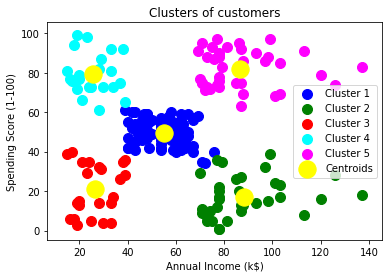
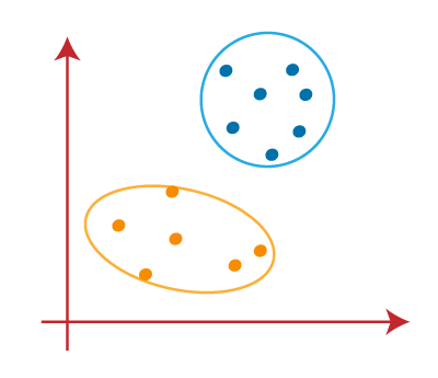
The output image is clearly showing the five different clusters with different colors. The clusters are formed between two parameters of the dataset; Annual income of customer and Spending. We can change the colors and labels as per the requirement or choice. We can also observe some points from the above patterns, which are given below:
- Cluster1 shows the customers with average salary and average spending so we can categorize these customers as
- Cluster2 shows the customer has a high income but low spending, so we can categorize them as careful.
- Cluster3 shows the low income and also low spending so they can be categorized as sensible.
- Cluster4 shows the customers with low income with very high spending so they can be categorized as careless.
- Cluster5 shows the customers with high income and high spending so they can be categorized as target, and these customers can be the most profitable customers for the mall owner.
Representing data and engineering features are important
steps in machine learning, as they can significantly impact the accuracy and
effectiveness of a machine learning model.
Representing data:
Data representation refers to the process of converting raw
data into a format that can be easily processed by a machine learning
algorithm. The choice of data representation can affect the accuracy of the
model, as different algorithms may perform better with different types of data.
Some common data representations used in machine learning
include:
Numerical data: numerical data is represented using
numbers, which can be continuous or discrete. This is the most common type of
data used in machine learning.
Categorical data: categorical data is represented
using discrete values, such as categories or labels.
Text data: text data can be represented using
bag-of-words models, where the frequency of occurrence of each word is used as
a feature, or using more advanced natural language processing techniques.
Image data: image data can be represented using pixel
values, or using more advanced techniques such as convolutional neural
networks.
Engineering features:
Feature engineering is the process of selecting and
transforming raw data into features that can be used by a machine learning
algorithm to make predictions. The choice of features can have a significant
impact on the accuracy of the model.
Some common techniques used in feature engineering include:
Normalization: scaling the data to a common range to
make it easier to compare.
Feature selection: selecting the most important
features based on statistical measures such as correlation or mutual
information.
Feature extraction: extracting new features from
existing ones, such as computing the mean or standard deviation of a set of
numerical values.
Encoding categorical variables: converting
categorical variables into numerical features that can be used by a machine
learning algorithm.
Overall, the process of representing data and engineering
features is an iterative one, and requires careful consideration and
experimentation to achieve the best results.
Types of Encoding in Machine Learning
There are several different encoding techniques used in
machine learning, each with its own strengths and weaknesses. Here are some of
the most common encoding techniques:
One-Hot Encoding: One-hot encoding is a technique
used to represent categorical variables as binary vectors. Each category is
represented as a binary vector, with a 1 in the position corresponding to the
category and 0s everywhere else.
Label Encoding: Label encoding is a technique used to
represent categorical variables as numerical values. Each category is assigned
a unique integer value, which is used to represent the category in the dataset.
Binary Encoding: Binary encoding is a technique used
to represent categorical variables as binary vectors. Each category is
represented as a binary vector, with a 1 in the position corresponding to the
bit value of the unique integer assigned to the category.
Count Encoding: Count encoding is a technique used to
represent categorical variables as numerical values. Each category is assigned
a value equal to the number of times it appears in the dataset.
Target Encoding: Target encoding is a technique used to
represent categorical variables as numerical values. Each category is assigned
a value based on the average target value for that category in the dataset.
Feature Hashing: Feature hashing is a technique used
to represent categorical variables as numerical values. Each category is hashed
to a numerical value using a hash function, which maps the category to a
fixed-size vector.
The choice of encoding technique depends on the specific
problem and dataset, and the performance of the model may vary depending on the
encoding technique used. It's important to experiment with different encoding
techniques and evaluate their impact on the model's performance.
One hot Encoding
Imagine you are a teacher in a classroom and you want to keep
track of your students' grades for different subjects. One way to do this is to
create a table where each row represents a student and each column represents a
subject. For example:
Student Math Grade Science Grade History Grade
Alice 85 92 77
Bob 76 89 92
Charlie 92 78 85
However, if you want to use this data in a machine learning
model, you will need to convert it to numerical format. One way to do this is
using one-hot encoding.
One-hot encoding is a technique used to represent
categorical variables as binary vectors. In this case, the subjects are
categorical variables, and we can create a binary vector for each subject. Each
vector has a length equal to the number of possible values for the variable,
and a value of 1 in the position corresponding to the student's grade for that
subject, and 0s everywhere else. For example, the one-hot encoding for the Math
column would be:
Student Math_76 Math_85 Math_92
Alice 0 1 0
Bob 1 0 0
Charlie 0 0 1
In this example, each row represents a student, and the
columns represent the possible grades for the Math subject. The value of 1 in
each column indicates the grade that the student received for that subject.
Overall, one-hot encoding is a useful technique for
representing categorical variables in a machine learning model. It allows us to
represent categorical data in a numerical format that can be easily processed
by machine learning algorithms.
Label Encoding
Imagine you are a teacher and you want to keep track of the
grades for different subjects that your students are taking. Let's say the
subjects are Math, Science, and History, and the possible grades are A, B, C,
D, and F. You want to represent this data in a way that can be used in a
machine learning model.
One way to do this is to use label encoding. With label
encoding, each category is assigned a unique integer value, which is used to
represent the category in the dataset. For example, you could assign the
following integer values to represent the grades:
A: 0
B: 1
C: 2
D: 3
F: 4
You could then create a table to represent the grades for
each student, where each column represents a subject and each value represents
the student's grade for that subject using the assigned integer values. For
example:
Student Math Science History
Alice 0 1 2
Bob 1 0 0
Charlie 2 3 1
In this example, each row represents a student, and the
columns represent the subjects. The values in each column represent the
student's grade for that subject using the assigned integer values.
Overall, label encoding is a useful technique for
representing categorical variables in a machine learning model. It allows us to
represent categorical data in a numerical format that can be easily processed
by machine learning algorithms. However, it's important to note that label encoding
can introduce an arbitrary order to the categories, which may not always be
meaningful or accurate.
Binary Encoding
Imagine you are a teacher and you want to keep track of the
grades for different subjects that your students are taking. Let's say the
subjects are Math, Science, and History, and the possible grades are A, B, C,
D, and F. You want to represent this data in a way that can be used in a machine
learning model.
One way to do this is to use binary encoding. With binary
encoding, each category is represented as a binary vector, with a 1 in the
position corresponding to the bit value of the unique integer assigned to the
category. For example, you could assign the following integer values to
represent the grades:
A: 0
B: 1
C: 2
D: 3
F: 4
You could then create a binary vector to represent the
grades for each subject, where each row represents a grade category and each
column represents the bit value of the assigned integer values. For example,
the binary vectors for the grades would be:
Grade Bit 0 Bit 1 Bit
2 Bit 3 Bit 4
A 1 0 0 0 0
B 0 1 0 0 0
C 0 0 1 0 0
D 0 0 0 1 0
F 0 0 0 0 1
In this example, each row represents a grade category, and
the columns represent the bit values of the assigned integer values. The value
of 1 in each column indicates the position corresponding to the bit value of
the assigned integer value for that grade.
You could then use these binary vectors to represent the
grades for each student, where each column represents a subject and each value
represents the binary vector for the student's grade using the assigned integer
values. For example:
Student Math Science History
Alice 1 0 0 0 0 0 1 0 0 0 0 0 1 0 0
Bob 0 1 0 0 0 1 0 0 0 0 1 0 0 0 0
Charlie 0 0 1 0 0 0 0 0 1 0 0 1 0 0 0
In this example, each row represents a student, and the
columns represent the subjects. The values in each column represent the binary
vector for the student's grade for that subject using the assigned integer
values.
Overall, binary encoding is a useful technique for
representing categorical variables in a machine learning model. It allows us to
represent categorical data in a binary format that can be easily processed by
machine learning algorithms. However, it can lead to a high dimensionality of
the dataset, especially when the number of categories is large, which can be
computationally expensive.
Count Encoding
Imagine you are a teacher and you want to keep track of the
grades for different subjects that your students are taking. Let's say the
subjects are Math, Science, and History, and the possible grades are A, B, C,
D, and F. You want to represent this data in a way that can be used in a
machine learning model.
One way to do this is to use count encoding. With count
encoding, each category is assigned a value based on the number of times it
appears in the dataset. For example, you could count the number of occurrences
of each grade category for each subject, and use these counts as the encoding
values. For example:
Grade Math Science History
A 1 2 1
B 2 1 0
C 0 1 2
D 1 0 0
F 0 0 1
In this example, each row represents a grade category, and
the columns represent the subjects. The values in each column represent the
count of the number of times the grade category appears for that subject.
You could then use these count encoding values to represent
the grades for each student, where each column represents a subject and each
value represents the count encoding value for the student's grade for that
subject. For example:
Student Math Science History
Alice 1 2 1
Bob 2 1 0
Charlie 0 1 2
In this example, each row represents a student, and the
columns represent the subjects. The values in each column represent the count
encoding value for the student's grade for that subject.
Overall, count encoding is a useful technique for
representing categorical variables in a machine learning model. It captures the
frequency of occurrence of each category, which can be informative in some
cases. However, it can be sensitive to outliers or imbalanced datasets, where
some categories may appear much more or much less frequently than others.
Target Encoding
Let's say you are a teacher and you want to predict the test
scores of your students based on their study habits. You have a dataset with
several features, including the student's name, their study time, the number of
books they read, and their favourite study location. In this example, the
target variable is the test score.
One way to encode the categorical feature of "favourite
study location" is to use target encoding. With target encoding, the
categorical variable is replaced with the average value of the target variable
(in this case, the test score) for each category. Here's an example:
Favourite Study Location Test
Score
Library 90
Home 85
Coffee Shop 80
Library 87
Coffee Shop 83
Home 92
Home 94
Coffee Shop 77
Library 88
Home 90
In this example, the favourite study location category is
encoded using target encoding. To do this, we compute the average test score
for each category:
Library: (90 + 87 + 88) / 3 = 88.33
Home: (85 + 92 + 94 + 90) / 4 = 90.25
Coffee Shop: (80 + 83 + 77) / 3 = 80
We can then replace the original values with these target
encoding values:
Favourite Study Location Test
Score
88.33 90
90.25 85
80 80
88.33 87
80 83
90.25 92
90.25 94
80 77
88.33 88
90.25 90
Now, the categorical variable "favourite study
location" is represented as continuous variables that can be used in a
machine learning model. Target encoding can help capture the relationship
between categorical variables and the target variable, and can be especially
useful when there are a large number of categories. However, it can also be
sensitive to outliers or imbalanced datasets, and requires careful validation
to avoid overfitting.
Feature Hashing
Let's say you are a teacher and you want to analyse the
comments that your students have written on their essays. You have a dataset
with several features, including the student's name, the essay topic, and the
comment they wrote. In this example, the comment is a text feature, which
cannot be used directly in a machine learning model. One way to represent this
text feature is to use feature hashing.
With feature hashing, the text feature is hashed into a
fixed number of numerical values, or "buckets". Each text feature is
hashed into the same number of buckets, so features with different lengths are
represented with the same number of numerical values. The hashing function used
is deterministic, so the same feature will always be hashed into the same
bucket.
Here's an example of how feature hashing works. Let's say we
have the following comments:
"Great job, keep up the good work!"
"Needs improvement, please see me after class."
"I appreciate your hard work and effort."
We want to hash each comment into 3 buckets. We can use a
hashing function to do this, such as the Python built-in hash() function.
Here's what the hashed values might look like:
Comment Hashed
Values
"Great job, keep up the good work!" [0, 1, 1]
"Needs improvement, please see me after class." [0, -1, 1]
"I appreciate your hard work and effort." [-1, 1, 0]
In this example, we used a hashing function to map each
comment to a fixed number of buckets, and represented each comment as a
fixed-length array of numerical values. This allows the text feature to be used
in a machine learning model as a continuous feature. Feature hashing can be
useful when dealing with high-dimensional text data, but can also result in
collisions, where different features are hashed to the same bucket, which can
reduce the accuracy of the model.
Cross Validation
Cross-validation is a technique used to evaluate the performance of a predictive model, such as a machine learning algorithm. The main goal of cross-validation is to estimate how well a model will generalize to new, unseen data. This is important because a model that performs well on the training data but poorly on new data is not very useful in practice.
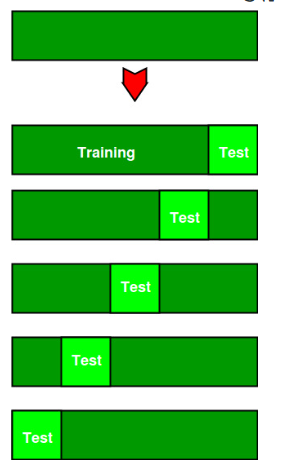
The basic idea behind cross-validation is to split the available data into two sets: a training set and a validation set. The model is trained on the training set and then evaluated on the validation set. However, to get a more accurate estimate of the model's performance, cross-validation involves repeating this process multiple times with different subsets of the data used as the training and validation sets.
The most commonly used type of cross-validation is k-fold cross-validation, where the data is divided into k subsets of equal size. The model is then trained on k-1 subsets and tested on the remaining subset. This process is repeated k times, with each subset used as the validation set once. The results of each fold are then averaged to give an overall performance estimate.

Cross-validation is an important tool for assessing the generalization performance of a model and can help prevent overfitting, where a model performs well on the training data but poorly on new, unseen data. By using cross-validation, we can get a more accurate estimate of a model's performance and make more informed decisions about which models to use in practice.
Advantages of Cross Validation:
- Overcoming Overfitting: Cross validation helps to prevent overfitting by providing a more robust estimate of the model’s performance on unseen data.
- Model Selection: Cross validation can be used to compare different models and select the one that performs the best on average.
- Hyperparameter tuning: Cross validation can be used to optimize the hyperparameters of a model, such as the regularization parameter, by selecting the values that result in the best performance on the validation set.
- Data Efficient: Cross validation allows the use of all the available data for both training and validation, making it a more data-efficient method compared to traditional validation techniques.
Disadvantages of Cross Validation:
- Computationally Expensive: Cross validation can be computationally expensive, especially when the number of folds is large or when the model is complex and requires a long time to train.
- Time-Consuming: Cross validation can be time-consuming, especially when there are many hyperparameters to tune or when multiple models need to be compared.
- Bias-Variance Tradeoff: The choice of the number of folds in cross validation can impact the bias-variance tradeoff, i.e., too few folds may result in high variance, while too many folds may result in high bias.
Categorize
the evaluation Matrix in detail in machine learning
In the context of machine
learning, evaluation matrices are used to measure the performance of a machine
learning model. These matrices can be broadly classified into the following
categories:
1. Classification Evaluation Matrices: These matrices are used to evaluate the
performance of classification models. Examples of classification evaluation
matrices include accuracy, precision, recall, F1-score, area under the receiver
operating characteristic curve (AUC-ROC), and area under the precision-recall
curve (AUC-PR).
2. Regression Evaluation Matrices: These matrices are used to evaluate the
performance of regression models. Examples of regression evaluation matrices
include mean absolute error (MAE), mean squared error (MSE), root mean squared
error (RMSE), R-squared (R2), and coefficient of determination.
3. Clustering Evaluation Matrices: These matrices are used to evaluate the
performance of clustering models. Examples of clustering evaluation matrices
include silhouette score, Calinski-Harabasz index, and Davies-Bouldin index.
4. Ranking Evaluation Matrices: These matrices are used to evaluate the
performance of ranking models. Examples of ranking evaluation matrices include
mean average precision (MAP), normalized discounted cumulative gain (NDCG), and
precision at k (P@k).
5. Anomaly Detection Evaluation Matrices: These matrices are used to evaluate the
performance of anomaly detection models. Examples of anomaly detection
evaluation matrices include true positive rate, false positive rate, precision,
recall, and F1-score.
6. Reinforcement Learning Evaluation Matrices: These matrices are used to evaluate the
performance of reinforcement learning models. Examples of reinforcement
learning evaluation matrices include average reward, convergence rate, and
exploration-exploitation trade-off.
It's important to note that the selection of the
appropriate evaluation matrix is dependent on the type of machine learning
problem being solved and the objectives of the model being evaluated.
Additionally, different evaluation matrices may be combined to provide a more
comprehensive evaluation of the model's performance.
What are machine learning Pipelines?
Machine learning pipelines are a series of interconnected processing steps designed to automate and simplify the process of building machine learning models. Pipelines typically consist of several stages, such as data preparation, feature engineering, model training, and evaluation.
The purpose of a pipeline is to provide a systematic and repeatable way to process data and train machine learning models. Pipelines can help ensure that data is processed consistently and accurately, and that models are trained using the same set of steps every time, reducing the risk of errors and variability in results.
Pipelines are also useful for managing the complexity of machine learning workflows. By breaking down the process into smaller, more manageable steps, pipelines make it easier to debug and troubleshoot issues that may arise during the training process.
Another advantage of machine learning pipelines is that they can be reused across different datasets and projects. Once a pipeline has been built and optimized for a particular task, it can be easily adapted and reused for other similar tasks, saving time and effort in the long run.
Overall, machine learning pipelines are an essential tool for building robust, efficient, and reproducible machine learning models that can be deployed in real-world applications.

The General Pipeline Interface in machine learning
The General Pipeline Interface (GPI) is a framework for building machine learning pipelines that enables developers to create complex workflows that can handle diverse data formats, feature engineering, and model selection.
The GPI allows developers to specify a sequence of processing steps, where each step takes an input and produces an output that is fed to the next step in the sequence. These steps can include data preprocessing, feature extraction, feature selection, and model training. The GPI also allows developers to define custom processing steps that can be incorporated into the pipeline.
The GPI provides a unified interface for building machine learning pipelines that can work with a variety of different data types and models. This means that developers can use the same pipeline for different datasets and models, which can save time and effort.
In addition, the GPI enables developers to experiment with different combinations of processing steps and model configurations to find the best pipeline for a given problem. This is done through hyperparameter tuning, where the developer can define a set of hyperparameters that control the behavior of the pipeline and use a search algorithm to find the best combination of hyperparameters.
Overall, the GPI provides a flexible and powerful framework for building machine learning pipelines that can handle diverse datasets and models, and enable developers to experiment with different configurations to find the best solution for a given problem.
Comments
Post a Comment